Thursday, December 30, 2010

Where on Google Earth-- New Year's Eve ed. (also #245)

Hello readers and happy new year!

Welcome to “Where on Google Earth" (WoGE for short). WoGE was started by Brian Romans (then blogging as “…or Something” and now as Clastic Detritus) in January of 2007 and is now close to entering its fourth year of geological adventure – virtually at least. I had fun with WoGE #244 as it was an adventure down the East African Rift. Coupled with the hint given by fellow geoblogger Andrew Alden (over at about.com), I raced over to eastern Africa, followed the rift valley north to south until I got to Lake Malombe with its sine-curve-shaped west shore. As a newcomer to this game myself, WoGE has allowed me to travel the virtual globe to parts that I probably would not have been to otherwise. Yeah, I'm busted! 


As victor of WoGE #244 the torch is hereby passed to me, and I get to set up the next WoGE challenge. Thus, I am pleased to offer WoGE #245. Veterans of this game know the rules, but for the benefit of newcomers to WoGE, here is how the game is played:

  1. Analyze the screen-capture (at the bottom of this post), and see if you can find where it is by using Google Earth.
  2. Write a comment to this post describing (a) the location (lat-long and/or specific locality) and (b) a sentence or two about the geology depicted in the image.
  3. The first person to correctly identify location and general geology of the image gets to host WoGE #246 on their geoblog – or create a geoblog and then host WoGE #246. Extra kudos if this challenge is solved before the year runs out!

Since this is a fairly straightforward challenge despite the small area pictured (I think), and to allow for WoGE newcomers a chance to get into the action, the Schott Rule is hereby invoked. Under this rule, previous winners must wait one hour after the contest starts to answer. 


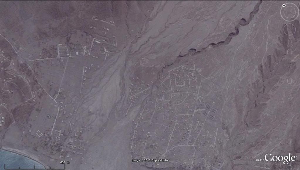
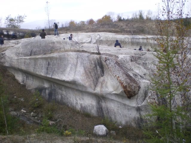
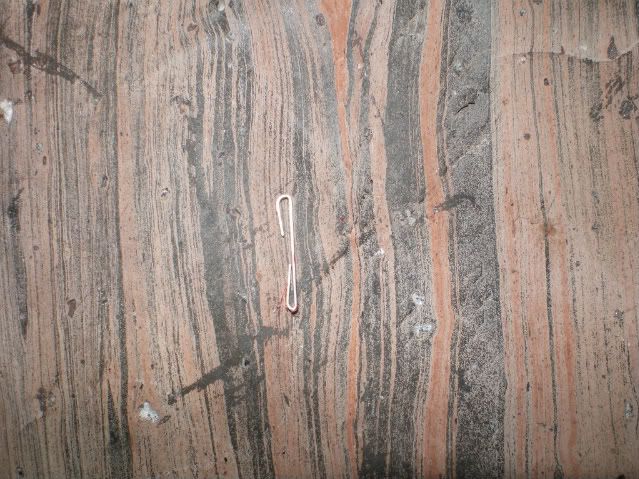
 Figure for WoGE # 245. Click to see a larger verson. This may be the first WoGE challenge using Google Earth v.6

Good luck, happy new year, and I'll see you in 2011! :-)


Posted on December 31st at 9:05 AM PST

Tuesday, December 21, 2010

End of Semester Wrap-up


Greetings readers!

After a couple of weeks or so taking care of wrapping up the fall semester, I have embarked on winter vacation in my other home near Portland, Oregon --Whew!. While my thesis field area is in the eastern Sierras of California, I think its time that I post some geologically noteworthy photographs in the area where I spend most of my time, in the National Capital Region of Canada. These photographs were taken on fieldtrips as a part of an introductory geology course that I was honoured to serve as a teaching assistant.


Glacially-carved “rat-tail” near the Cantley Quarry, north of Gatineau, Quebec. A relatively resistant xenolith within less resistant marble (both of Grenville affinity) provides good information regarding the trajectory of glacial ice movement from the Laurentide Ice Sheet. In this photo, the ice moved right-to-left.


Glacial striations in both the xenolith and the enclosing marble from the Cantley Quarry. The right-margin of the xenolith resembles “slicken-fibres.” Unsure if it was from the glaciations or from the Grenville orogeney (thoughts?) Yellow-part of the pen points in the direction from where the ice flowed.


Photo showing an unconformity between the Precambrian Grenville gneiss, below and the Paleozoic Nepean Sandstone above nearby. The gneiss is ~1 Ga (billion years old) whereas the Nepean sandstone is ~500 Ma (million years old). Thus, about a half-billion years of earth history in the Ottawa Valley is missing. Photo was taken beside a road in Parc Lac Beauchamp in Gatineau, Quebec.

Have a great holiday!

All photos (c) by Cole Kingsbury

Friday, December 10, 2010

Flow Banding: A Short Primer (also my first crack at research blogging)


Happy Weekend everyone!

Because the title of my blog is “Chaotically Flow-Banded,” I think its high time that I blog about, you know, flow banding! Flow banding is a pervasive feature that can be found in many different lava flows and domes throughout the world. Because of this fact, they can often be used to characterize the internal structure of many different lava flows as they extruded and then solidified. In other words volcanologists can use flow bands much like how structural geologists use sedimentary successions and metamorphic fabrics to help characterize regional deformation patterns.

But what are flow bands? Simply put, flow bands are rhythmically sequenced "layers" which are distinct compared to adjacent "layers". Flow bands can vary in thickness on scales from a few microns to 10s of centimeters. Banding can be defined in many different ways, however most are not defined by distinct compositional changes between bands, but instead by texture or oxidation states. For example, at Obsidian Dome, where I am currently completing a thesis, flow bands are chiefly defined by microlite densities (see figure below). In other flows like the Mayor Island flow in New Zealand, flow banding is defined by vesicularity (see fig. 5 in Gonnermann and Manga, 2005).

Photomicrograph showing microlite-defined, horizontally-oriented flow banding. Darker bands are denser in microlites. 10x magnification. Brownish feature on right is a spherulite.

Flow-banding is perhaps one of my favourite things to look at in the field and in hand sample – especially when it gets deflected around phenocrysts, as this is beautifully shown below.


Close-up photo of spectacularly flow-banded obsidian from Obsidian Dome as accentuated by surficial weathering of iron oxide (likely from the microlite-rich bands of ferromagnesian minerals). Staple is ~1 cm wide. To the right of the lower staple hook, flow bands are deflected by a phenocryst.  
 
Have a great weekend, and please comment!
 
Reference:

Gonnermann, H. M. and Manga, M., 2005, Flow banding in obsidian: A record of evolving textural heterogeneity during magma deformation. Earth and Planetary Science Letters, 236 (1-2), p. 135-147.

All photos (c) 2010 by Cole Kingsbury

Saturday, December 4, 2010

Photographic Geology

      One of the amazing aspects of geology is the ability to travel while simultaneously doing a job -- or is it really a job when you have so much fun? Obsidian Dome (and the entire Mono / Long Valley area for that matter) is a volcanic playground replete with compelling sites like Panum Crater , Mammoth Mountain , Hot Creek, and the infamous "CO2 Tree Kill" area at Horseshoe Lake. All of these site -- and more -- are quite photogenic.

      To start off, I will tackle Obsidian Dome, (or as I like to refer to it "my baby" or "the sid"). Since I am studying how Obsidian Dome cooled from phase-observations and textural analysis, it is vitally important to make many observations at the macroscopic all the way down to microscopic scales. Because I had only ~7 days to take field data, I basically had enough time to "skim the surface." Nonetheless, each site I visited has a unique story. I have included three images below that exemplify some of the more interesting patterns found at Obsidian Dome.


This "drip feature" is interesting. Considering that rhyolite melt is quite viscous, it seems somewhat out of character. On the other hand, and perhaps a more likely scenario, it could be a tight fold which would indicate ductile deformation.


The above two photos are taken from a "crease structure" on Obsidian Dome. The upper photo shows the general scale of the structure (backpack for scale). The bottom photo is a close-up of a particularly interesting feature in the wall of the crease structure, Canadian nickel for scale. Note the disharmonic folding of a pronounced flow band. Flow banding is a pervasive feature of Obsidian Dome among other extrusions, (it is also how I arrived at my blog name). I will touch more on flow banding in a later post. But for now, enjoy these photos, and have a great weekend!

All photos (c) 2010 by Cole Kingsbury